Chapter 3

Modelling Future Climate Change

This chapter describes what Earth system models are and how they are used. Model-based projections of climate change at a global scale are presented, along with a discussion of the global carbon budget and methods to downscale coarse resolution global model projections to finer spatial scales.

Recommended citation

Flato, G., Gillett, N., Arora, V., Cannon, A. and Anstey, J. (2019): Modelling Future Climate Change; Chapter 3 in Canada’s Changing Climate Report, (ed.) E. Bush and D.S. Lemmen; Government of Canada, Ottawa, Ontario, p. 74-111.

Authors

  • Greg Flato (Environment and Climate Change Canada)
  • Nathan Gillett (Environment and Climate Change Canada)
  • Vivek Arora (Environment and Climate Change Canada)
  • Alex Cannon (Environment and Climate Change Canada)
  • James Anstey (Environment and Climate Change Canada)
Figure-3.1
View details
Figure-3.2
View details
Figure-3.3
View details
Figure-3.4
View details
Figure-3.5
View details
Figure-3.6
View details
Figure-3.7
View details
Figure-3.8
View details
Figure-3.9
View details
Figure-3.10
View details

Chapter Key Messages

FUTURE CHANGE AND CLIMATE FORCING

Emissions of greenhouse gases from human activity, particularly carbon dioxide, will largely determine the magnitude of climate change over the next century. Therefore, reducing human emissions will reduce future climate change.

MODELLING THE RESPONSE OF THE CLIMATE SYSTEM TO EXTERNAL FORCING

In the near term (to approximately 2040), projected warming will be similar under all emission pathways. But by the late 21st century, the differences between possible emission pathways will have a considerable effect. Available estimates indicate that the global climate will warm by an additional 1°C (for a low emission scenario) to 3.7°C (for a high emission scenario). Scenarios that would limit warming to an additional 1°C or less require rapid and deep emission reductions.

CUMULATIVE CARBON AND GLOBAL TEMPERATURE CHANGE

Global temperature change is effectively irreversible on multi-century timescales. This is because the total amount of carbon dioxide emitted over time is the main determinant of global temperature change and because carbon dioxide has a long (century-scale) lifetime in the atmosphere.

REGIONAL DOWNSCALING

Climate projections are based on computer models that represent the global climate system at coarse resolution. Understanding the effects of climate change for specific regions benefits from methods to downscale these projections. However, uncertainty in climate projections is larger as one goes from global to regional to local scale.


Summary

This chapter provides an overview of Earth system models and how they are used to simulate historical climate and to make projections of future climate. Historical simulations allow models to be evaluated via comparison with observations, and these show that models are able to reproduce many aspects of observed climate change and variability. They also allow experiments to be conducted in which human and natural causes of climate change can be identified and quantified. In order to make future projections, it is necessary to specify future emissions, or concentrations of greenhouse gases and aerosols, as well as future land-use change. Owing to uncertainty regarding future human activity (in particular, the extent to which ambitious emission reductions will be implemented), a range of future scenarios must be used. Results from future climate projections are discussed, along with sources of confidence and uncertainty. On average, the models project a future global mean temperature change (relative to the 1986–2005 reference period) of about 1°C for the low emission scenario (Representative Concentration Pathway [RCP] 2.6) and 3.7°C for the high emission scenario (RCP 8.5) by the late 21st century, with individual model results ranging about 1°C above or below the multi-model average. This change is over and above the 0.6°C change that had already occurred from 1850 to the reference period. The low emission scenario (RCP2.6) is consistent with limiting the global temperature increase to roughly 2°C and is therefore roughly compatible with the global temperature goal agreed to in the Paris Agreement. This scenario requires global carbon emissions to peak almost immediately and reduce to near zero well before the end of the century.

Regardless of the global mean surface temperature level attained when emissions become net zero, temperature will remain at about that level for centuries. In other words, global temperature change is effectively irreversible on multi-century timescales. The relationship between cumulative emissions of carbon dioxide (CO2) and global mean surface temperature provides a simple means of connecting emissions from fossil fuels — the main source of anthropogenic CO2 — to climate change. It also leads to the concept of a carbon emissions budget — the amount of carbon that can be emitted before temperatures exceed a certain value. The Intergovernmental Panel on Climate Change (IPCC, 201424) has assessed that, to have a 50% chance of keeping global warming to less than 2°C above the pre-industrial value, CO2 emissions from 2011 onward would have to remain below 1300 billion tonnes of CO2 (GtCO2), roughly equal to what has already been emitted since the beginning of the Industrial Era. For a 50% chance of keeping the temperature increase to less than 1.5°C, emissions from 2011 onward would have to be limited to 550 GtCO2. It must be noted that estimation of carbon budgets, especially for low temperature targets, is a rapidly developing area of research, and updated budgets will be assessed in the near future.

The chapter concludes with a discussion of downscaling methods, that is, methods to transform global Earth system model results into more detailed, local information better suited to impact studies. Downscaled results are often used in impact studies, but users must keep in mind that the enhanced detail provided does not necessarily mean added value, and that uncertainty is larger at smaller spatial scales.

3.1

Introduction

Future climate change will be driven primarily by human emissions of greenhouse gases (GHGs). Emissions of aerosols (airborne particles) collectively cool the climate and so offset some climate warming, but this effect is projected to decrease in the future as aerosol emissions decline. To understand the effects of these drivers on the climate, scientists use models — complex computer simulations of the climate system. Models are used to make projections of future climate, based on future scenarios of GHG and aerosol forcing. These models are developed and used at climate research institutions around the world, and results from multiple models allow us to estimate uncertainty and overall confidence in future projections. While Earth system models can simulate the climate system’s response to human emissions of GHGs, they cannot predict future human activities. Therefore, projections are made using various scenarios, or pathways, of future GHG concentrations, aerosol loading and land-use change (climate forcing agents; see Chapter 2, Section 2.3.1). These pathways are described in Section 3.2. In Section 3.3, Earth system models are briefly described, along with global-scale projections of future climate and sources of uncertainty in such projections. While all forcing agents affect climate, carbon dioxide (CO2) is the main determinant of long-term global temperature change. Section 3.4 describes the relationship between CO2 emissions and global temperature change — a relationship that is important in developing policies on temperature targets and on global emission reductions. This section also discusses why climate change is irreversible, due to the long lifetime of CO2 in the climate system. Finally, Section 3.5 discusses how global model results can be “downscaled” to provide more detailed regional information more suitable for impact assessment and adaptation planning.

3.2

Future climate change and climate forcing

Key Message 1

Emissions of greenhouse gases from human activity, particularly carbon dioxide, will largely determine the magnitude of climate change over the next century. Therefore, reducing human emissions will reduce future climate change.

Projections of future climate change require projections of future climate forcing — the external drivers of change such as GHGs and aerosols. These projections, in turn, arise from scenarios of future GHG and aerosol emissions, which are based on varying assumptions about how human activities, such as fossil fuel consumption and land use, will change. Future emission scenarios are typically developed using integrated assessment models, which combine economic, demographic, and policy modelling with simplified physical climate models to make projections of population growth, economic development, land use, and the implications of different policy options on climate-relevant emissions. As there is large uncertainty in the social and economic aspects of such projections, a range of scenarios is generally provided, ranging from those in which emissions are aggressively reduced to those with limited actions taken to mitigate emissions.

The projections described in the IPCC Fifth Assessment (see Chapter 1) were based on a suite of future forcing scenarios called Representative Concentration Pathways (RCPs) that cover the period from 2006 onward (van Vuuren et al., 201154). The RCPs are identified by a number indicating the change in radiative forcing — the imbalance between the solar radiation entering the climate system and the infrared (longwave) radiation leaving it caused by greenhouse gases and other external drivers (see Chapter 2, Section 2.3.1) — by the end of the 21st century. RCP2.6 represents a low emission pathway with a change in radiative forcing of roughly 2.6 W/m2, RCP4.5 and RCP6 represent intermediate emission pathways, and RCP8.5 represents a pathway with continued growth in GHG emissions, leading to a radiative forcing of roughly 8.5 W/m2 at the end of the century. In this report, we will refer to climate scenarios based on RCP2.6 as “low emission scenarios,” those based on RCP4.5 and RCP6 as “medium emission scenarios,” and those based on RCP8.5 as “high emission scenarios.” For each RCP, the integrated assessment models provide a comprehensive time series of emissions and concentrations of individual GHGs (CO2, methane [CH4], nitrous oxide [N2O], chlorofluorocarbons, etc.), along with aerosol emissions and land-use change. All of these forcings are inputs to Earth system models, which then simulate the future response of the climate system, including biogeochemical feedbacks, to these external forcing scenarios.

The RCPs supersede the so-called “SRES scenarios” (Nakicenovic et al., 200040), which served as the basis for model runs reported in the IPCC Fourth Assessment Report. Although there are differences in detail, the SRES A2 forcing scenario is roughly comparable to RCP8.5, the SRES A1B scenario is roughly midway between RCP6 and RCP8.5, and SRES B1 is roughly comparable to RCP4.5 (e.g., Burkett et al., 20142). There was no SRES forcing scenario comparable to RCP2.6. These forcing scenarios are updated every few years, and new shared socioeconomic pathways (building upon the RCPs) will be used in model runs that will feed into the upcoming IPCC Sixth Assessment (e.g., Riahi et al., 201741).

In all cases, CO2 is the largest contributor to the historical and projected change radiative forcing, followed by CH4 and N2O (Myhre et al., 201339; Collins et al., 20135). This means that future changes in human emissions of CO2 will largely determine future climate.

An illustration of aspects of the RCPs is shown in Figure 3.1. It is important to note that no likelihoods are ascribed to these future forcing scenarios — they are all deemed plausible, although, as emissions continue to increase, low emission pathways become more difficult to achieve (e.g., Millar et al., 201737). The spread across the RCPs represents some measure of our uncertainty about how socioeconomic factors may change in the future, especially how aggressively humans will pursue emission mitigation, and therefore the pace at which humans will continue to drive climate change. The low emission (RCP2.6) scenario is consistent with limiting global temperature increase to roughly 2°C above the pre-industrial value (see Section 3.3.3) and is therefore roughly compatible with the global temperature goal agreed to in the Paris Agreement (UNFCCC, 201553). This scenario requires global CO2 emissions to peak almost immediately and reduce to near zero well before the end of the century. Global annual CO2 emissions reached about 10 Gt of carbon (about 37 GtCO2) in 2017 (Le Quéré et al., 201730)

Figure-3.1

Underlying features of the Representative Concentration Pathways

This figure provides coloured line plots showing the value of various quantities as a function of time from 2000 to 2100. In each case, results are shown for four Representative Concentration Pathways (RCPs): RCP2.6 is a low emission pathway; RCP4.5 and RCP6.0 are medium emission pathways; RCP8.5 is a high emission pathway. The first panel shows global population, which rises from 6 billion to about 9 billion in the three lowest scenarios, and to about 12 billion in RCP8.5. The second panel shows global gross domestic product (GDP). For RCP6.0 and RCP8.5, GDP increases about five-fold over the 21st century, whereas for RCP2.6 and RCP4.0, the increase is about eight-fold. The next panel shows global primary energy consumption, which starts at about 500 exajoules (EJ) in 2000 and increases to about 800 EJ by 2100 for RCP2.6, RCP4.0, and RCP6.5. For RCP8.5, the value at year 2100 is about 1700 EJ. The next panel shows global oil consumption (also in EJ). In this case, RCP4.5 and RCP6.0 show modest increase from about 150 EJ in year 2000 to about 200 EJ in year 2100. RCP8.5 shows a strong increase to about 300 EJ by year 2070, followed by rapid reduction back to just over 150 EJ at year 2100. RCP2.6 has oil consumption increasing slightly after 2000 and the declining fairly steadily to a value of about 50 EJ by year 2100. The next three panels show emissions of the three most important greenhouse gases — carbon dioxide, methane, and nitrous oxide. In all cases, emissions rise most rapidly under RCP8.5 and decline in RCP2.6, with the other two pathways in between. The last three panels show atmospheric concentrations of these three greenhouse gases. Under RCP8.5, the concentration of all three major gases increases throughout the century in response to rising emissions, with carbon dioxide concentrations increasing from roughly 375 parts per million (ppm) at the beginning of the century to over 900 ppm by 2100. Under RCP2.6, the concentration of carbon dioxide peaks at about 450 ppm at mid-century and then declines slightly to just over 400 ppm by 2100.
Figure-3.1

Socioeconomic (top row), energy intensity (second row), greenhouse gas emissions (third row), and ultimately greenhouse gas concentration (bottom row) scenarios underlying the Representative Concentration Pathways (RCPs) used to drive future climate projections. The light grey shading indicates the 98th percentile and the dark grey shading the 90th percentile of the underlying databases.

Source

Reproduced from van Vuuren et al. (2011), where further details are provided.


Section summary

In summary, projections of future climate require projections of future forcing from GHGs, aerosols, and land-use change, which in turn depend on projections of future population and energy consumption. CO2 is the largest contributor to human-induced climate forcing, and so CO2 emissions and the extent to which they grow or decline will largely determine future climate.

3.3

Modelling the response of the climate system to external forcing

Key Message 1

In the near term (to approximately 2040), projected warming will be similar under all emission pathways. But by the late 21st century, the differences between possible emissions pathways will have a considerable effect. Available estimates indicate that the global climate will warm by an additional 1°C (for a low emission scenario) to 3.7°C (for a high emission scenario). Scenarios that would limit warming to an additional 1°C or less require rapid and deep emission reductions.

3.3.1

Earth system models

Earth system models are based on a mathematical representation of the behaviour of the atmosphere, ocean, land surface, and cryosphere. They simulate a virtual planet using powerful supercomputers, allowing scientists to probe the connections between various physical and biogeochemical processes, e.g., how the ocean takes up heat and carbon, stores and then redistributes it. Two main ways such models are used are (1) to compare simulations with and without historical forcings to determine human versus natural forcing effects, and (2) to simulate future climate in response to various forcing scenarios.

Earth system models have some features in common with global weather-prediction models (used to make daily weather forecasts) but do not depend on the use of observations as inputs and typically operate at somewhat lower spatial resolution (i.e., the level of spatial detail is often limited to features with scales of a hundred kilometres or larger). The lower resolution is necessitated by the computing demand of the long simulations that are required. Simulations begin with the historical period (from 1850 to present), driven by observationally based climate forcing (e.g., historical changes in GHG concentrations), and then continue into the future, using different forcing scenarios (such as those described in the previous section) out to year 2100 or further (Figure 3.2).

Figure-3.2

Building an Earth system model

This figure is a schematic showing the processes included in an Earth system model (ocean transport, atmospheric mixing, clouds, precipitation, runoff, shortwave and longwave radiation, etc.). The figure also illustrates examples of the mathematical equations used to describe this complex system and the global numerical grid on which computer calculations are performed.
Figure-3.2

Schematic illustration of the processes included in an Earth system model, and the way in which mathematical equations describing physical processes are solved on a three-dimensional grid.

Source

Climate Research Division, Environment and Climate Change Canada.

Earth system models represent an evolution from earlier physical climate models (representing the coupled atmosphere, ocean, land, and sea ice components of the climate system) to models that go beyond this with explicit representation of the carbon cycle (Flato, 201113; Flato et al., 201314). Including carbon and other biogeochemical cycles in the models allows simulation of global interactions among ecosystems, carbon, and climate, as well as several terrestrial processes that occur at high latitudes. Changes to snow and sea ice can cause positive (amplifying) snow/ice albedo feedbacks in the climate system (Euskirchen et al., 201612; Kashiwase et al., 201726; see Chapter 2, Box 2.4). As temperatures increase, the spatial extent of snow and sea ice declines, reducing the reflectivity of land and oceans, allowing more solar radiation to be absorbed, and hence further increasing temperatures. This feedback makes an important contribution to the higher rate of warming in the Arctic region, called Arctic amplification (FAQ 3.1; see Section 3.3.3). The models can also simulate increased growth of vegetation at northern high latitudes in response to a warming climate, an effect that may reduce the land surface albedo and affect the exchange of energy and water between the land and the atmosphere (Forkel et al., 201615). Changes in permafrost in response to changing climate — leading to changes in hydrological conditions and CH4 release (Schuur et al., 200844) — are also now included in some models.

How do we know that models are accurately projecting future climate? One method of measuring whether models can realistically represent the complex interconnections among climate processes is to gauge their ability to reproduce past changes. Simulations using observationally based historical forcing from 1850 onward provide the opportunity to directly compare model results to observations. The IPCC Assessment Reports have traditionally included a chapter devoted to this type of model evaluation (e.g., Flato et al., 201314), and these provide a synthesis of the large number of scientific papers on model performance. Figure 3.5 provides one example of model evaluation, comparing the annual global mean surface air temperature from several different sources with simulations from 36 different models that participated in the fifth phase of the Coupled Model Intercomparison Project (CMIP5; see Box 3.1). As the figure shows, Earth system models are able to reproduce the observed long-term increase in temperature (heavy black lines), along with the sporadic cooling that follows large explosive volcanic eruptions. The magnitude of natural year-to-year variability is also well simulated (thin lines), although one does not expect individual ups and downs to coincide (as each model simulates its own internal variability). The heavy red line in the figure shows the multi-model average, which is an approximation of the response of the climate system to external forcing (changing GHG concentrations and aerosol amount, land-use change, variations in solar irradiance, and volcanic aerosol), upon which internal variability is superimposed. The difference between observed temperature and the multi-model average from roughly 2000 onward has been extensively analyzed (e.g., Fyfe et al., 201617) and is due to a combination of small errors in the observational record, decadal timescale internal variability, and incomplete early 21st century volcanic forcing in the models (see Chapter 2, Section 2.3.3).

Figure-3.5

Evaluating model performance against observations

This figure shows time series of annual global mean surface air temperature from 1850 to 2012. Values are shown as anomalies (differences) relative to the 1986–2005 average, so that changes over the period are clearly visible. There are many coloured lines showing results from 36 different global climate models, with a heavy red line showing the multi-model average. In addition, three observationally based time series are shown. In all cases, there is year-to-year variability, with a rather modest increase up to about 1960, followed by an evident, more rapid, increase. The observed values generally lie within the spread of the model results. Both models and observations start with a negative anomaly between 0°C and −0.5°C in the 1800s and end with a positive anomaly between about 0.4°C and 0.9°C in 2012. For almost the entire period, the multi-model average is very close to the observed value, but for the last decade or so it is slightly above.
Figure-3.5

Global annual mean surface air temperature anomalies from 1850 to 2012 (anomalies are computed relative to the 1961–1990 average shown by yellow shading). The heavy black lines represent three different reconstructions of temperature based on observations. Each of the thin coloured lines represents a simulation from one of 36 climate models. The heavy red line indicates the multi-model average. The overall warming trend is evident in both observations and simulations, particularly since about 1960, and both show cooling following large volcanic eruptions (vertical dashed lines).

Source

Adapted from Flato et al. (2013), Figure 9.8.

3.3.2

Sources of confidence and uncertainty

Confidence in climate model projections arises from many sources. First, climate models are solidly based on physical laws and scientific understanding of physical processes. Second, climate model results are evaluated in detail by comparing model output to observations, as described in Section 3.3.1. The model evaluation chapter in the most recent IPCC Assessment report provides many examples (Flato et al., 201314). Third, some of the models used to make climate projections are also used to make seasonal climate predictions whose skill is routinely evaluated (e.g., Kirtman et al., 201328, Merryfield et al., 201336; Sigmond et al., 201347; Kharin et al., 201727).

There are, however, uncertainties that have to be considered when using model projections. These uncertainties stem from the fact that models cannot simulate all physical processes exactly (and therefore must make approximations), and from internal variability in both the simulated and the real climate system (see Chapter 2, Box 2.5). The uncertainty due to approximations of physical processes can be reduced, in principle, and models continue to improve in this regard (Flato et al., 201314). However, it is impossible to reduce the uncertainty from internal variability that is superimposed on the underlying forced climate change. In addition, there is uncertainty about what future climate forcing (e.g., future GHG emissions) will be, which is accounted for by making projections with a range of forcing scenarios. These sources of uncertainty vary in importance depending on the time and space scale under consideration — generally, uncertainties diminish at larger spatial scales as internal variability “averages out” to a certain degree when one considers larger regions (e.g., Hawkins and Sutton, 200921). This also means that uncertainty is larger when one looks at small regions or specific locations. In addition, at longer time scales (say, by the end of the 21st century), uncertainty is dominated by differences in the forcing scenarios and internal variability is, by comparison, much smaller.

3.3.3

Global-scale climate projections

As described in Section 3.2, climate projections are a result of driving climate models with different future forcing scenarios (RCPs, in the case of CMIP5). These projections include the response of the climate system to external forcing (e.g., changing GHG concentrations), internal variability, and uncertainties associated with differences between models. These effects can be separated, to some extent, by drawing upon projections from multiple models (e.g., Collins et al., 20135). The multi-model average provides an estimate of the response of the climate system to forcing, since internal variability and model differences are “averaged out” to a large extent (see Box 3.2). The upper panel of Figure 3.6 shows the change over time in global mean surface air temperature, as simulated by the CMIP5 models, spanning the period from 1950 to 2100. The heavy lines indicate the multi-model average, and the shaded band represents the range of model results around this average. Within this shaded band, each individual model result would look like one of the individual coloured lines in Figure 3.5, but for clarity this collection of individual lines is shown as a shaded band. The high emission scenario (RCP8.5) results are shown by the red line and the orange shaded band, whereas the low emission scenario (RCP2.6) results are shown by the blue line and the blue shaded band.

There are two key points illustrated in the upper panel of Figure 3.6. First, when looking at projected climate change, the spread across models (the vertical extent of the shaded bands) is smaller in the near term (to around 2040) than it is toward the end of the 21st century, indicating that model uncertainty has a larger effect further into the future. (Internal variability also contributes to the width of the shaded bands, as described previously, but the size of this contribution is not expected to change significantly in the future.) Second, the differences among forcing scenarios are small in the near term, but become large toward the end of the 21st century (as illustrated by the growing separation between results for the low emission scenario [RCP2.6] and high emission scenario [RCP8.5]). For simplicity, the medium emission scenarios (RCP4.5 and RCP6.0) are not shown in the main part of the figure, but their end-of-century results are shown on the right-hand side of the top panel for comparison.

The spatial patterns of projected temperature and precipitation change are shown in the bottom panel of Figure 3.6. The large difference in mean change between the high and low emission scenarios is clearly evident in the maps (darker colours indicate larger change), but there is a marked similarity in pattern. For temperature, changes are larger over land than over the adjacent ocean, and are larger at high latitudes, particularly over the Arctic, an illustration of Arctic amplification. As a result, projected warming in Canada is roughly double the global mean. For precipitation, the pattern of change is more complex, with the polar and equatorial regions projected to have increased annual precipitation, whereas precipitation decreases are projected for much of the subtropics (roughly 24° to 35° north and south latitude). For southern Canada, the projected change in precipitation is rather small, but projected increases are larger further north. (Changes in annual mean precipitation do not translate directly into changes in seasonal snow cover or water availability, as discussed in Chapter 5 and Chapter 6.)


The spatial patterns of projected temperature and precipitation change are shown in the bottom panel of Figure 3.6. The large difference in mean change between the high and low emission scenarios is clearly evident in the maps (darker colours indicate larger change), but there is a marked similarity in pattern. For temperature, changes are larger over land than over the adjacent ocean, and are larger at high latitudes, particularly over the Arctic, an illustration of Arctic amplification. As a result, projected warming in Canada is roughly double the global mean. For precipitation, the pattern of change is more complex, with the polar and equatorial regions projected to have increased annual precipitation, whereas precipitation decreases are projected for much of the subtropics (roughly 24° to 35° north and south latitude). For southern Canada, the projected change in precipitation is rather small, but projected increases are larger further north. (Changes in annual mean precipitation do not translate directly into changes in seasonal snow cover or water availability, as discussed in Chapter 5 and Chapter 6.)

Figure-3.6

Global climate projections

The upper panel of this figure shows the anomaly in global mean surface air temperature, as simulated by Earth system models covering the period 1950 to 2100. Over the historical period (1950–2005), the multi-model average is shown as a heavy black line surrounded by a light grey band, indicating spread across the multi-model ensemble. For the future, a heavy blue line, surrounded by blue shading, illustrates the model projections under RCP2.6, and it shows mean warming of about 1°C by the late 21st century relative to the 1986–2005 reference period. For RCP8.5, warming is projected to be about 3.7°C above the reference period by late century, with a larger range across models. The lower panel of the figure shows global maps of temperature and precipitation change, illustrating the spatial pattern of the multi-model mean results described for the upper panel. For both temperature and precipitation, results are shown for RCP2.6 and RCP8.5. The map of temperature change for RCP2.6 shows increases of roughly 0.5°C to 1°C in the tropical regions and increases of over 2°C in the Arctic. There is only one small region south of Greenland that shows a very small decrease in temperature. For RCP8.5, there is much larger warming projected everywhere, with values of around 2°C to 3°C over the Southern Hemisphere oceans and over 7°C in the high Arctic. In all cases, warming over land is larger than over the adjacent ocean. The map showing projected precipitation change indicates both increases and decreases, depending on location. For RCP2.6, the changes are typically between a 10% increase and a 10% decrease, except for a narrow band along the equator and the area over the Arctic Ocean, which have increases of about 20%. For RCP8.5, the changes are much larger, and the spatial pattern is much more striking. Precipitation decreases of 20% or more are projected over the subtropical ocean regions and the Mediterranean, whereas increases of 50% or more are shown over the equatorial Pacific, Indian Ocean, central Africa, and both the Arctic and Antarctic.
Figure-3.6

The upper panel shows the multi-model annual global mean surface temperature change relative to a historical reference period (1986–2005) for a range of emission scenarios. The shaded bands indicate the 5%–95% spread across the multi-model ensemble. The lower panels show the multi-model mean projected change by late century (the 2081–2100 average minus the 1986–2005 average) for annual (b) mean surface air temperature and (c) precipitation for the low emission scenario (RCP2.6) and the high emission scenario (RCP8.5).

Source

Adapted from IPCC (2013) Figures SPM.7 and SPM.8 and Collins et al. (2013).

On average, the models project a future global mean temperature change (relative to the 1986–2005 reference period) of about 1°C for the low emission scenario (RCP2.6) and 3.7°C for the high emission scenario (RCP 8.5) by the late 21st century, with a 5%–95% range of about 1°C above and below the multi-model average. This change is over and above the 0.6°C change that had already occurred from 1850 to the reference period. Therefore, the average projected change under the low emission scenario is consistent with the global temperature target in the Paris Agreement of limiting global warming to between 1.5°C and 2.0°C, although the projected range from all models extends both below and above this target. The low emission (RCP2.6) scenario requires emissions of CO2 to peak almost immediately and reduce to near zero before the end of the century. Recent studies (e.g., Millar et al., 201737) provide more detailed analysis of scenarios that will limit warming to 1.5°C, and these also involve very rapid and deep emission reductions.

More details regarding future projections, with a focus on Canada, are provided in other chapters of this report. Confidence in climate change projections varies by region and by climate variable. So, for example, confidence in temperature change is higher than confidence in precipitation change. This is in large part because temperature change is a direct consequence of radiative forcing, whereas precipitation change is affected by a number of complex interactions, including changes in the water-holding capacity of a warming atmosphere, in global atmospheric circulation, in evaporation, and in other factors (e.g., Shepherd, 201446) (see Chapter 4). Changes in snow and ice are a consequence of changes in both temperature and precipitation and are discussed in more detail in Chapter 5. Freshwater availability (see Chapter 6) and ocean changes (see Chapter 7) are also affected by changes in temperature and precipitation, as well as by other factors.

3.3.4

Compatible emissions

Earth system models can be run in two different ways: one in which GHG concentrations are set and another in which GHG emissions are set (both are available as part of the RCP datasets). Concentration-driven simulations allow scientists to assess the difference, from one model to another, in how the climate responds to identical changes in GHG concentrations in the atmosphere. This helps separate the response of the climate system to a change in forcing (e.g., change in GHG concentrations) from the effect of carbon-cycle feedbacks involving the terrestrial and oceanic biospheres. The response of these natural carbon sinks to atmospheric CO2 levels and to climate change will influence anthropogenic emissions compatible with a given CO2 pathway. Therefore, an interesting aspect of these concentration-forced simulations is that global anthropogenic emissions can be computed — emissions that are compatible with the prescribed concentration pathway (e.g., Jones et al., 201325). The range in compatible CO2 emissions between different models provides a measure of the uncertainty inherent in representing carbon-cycle feedbacks in models. Figure 3.7 illustrates results from compatible emission calculations and shows that, while there is some variation, this group of models is consistent. For the RCP 2.6 scenario in which temperature is stabilized below about 2°C, the models have compatible emissions that start reducing immediately and reach near zero well before the end of the century.

Figure-3.7

Carbon dioxide concentrations and compatible emissions under the four Representative Concentration Pathways

A two-part figure showing carbon dioxide concentrations and compatible emissions over the historical period and in the future under the four Representation Concentration Pathways (RCPs). The upper panel shows observed carbon dioxide concentration increasing from around 280 ppm in 1860 to around 380 ppm in 2005, followed by its future evolution under four different RCPs, ranging from a strong increase to about 940 ppm in RCP 8.5, to a small increase and subsequent decline to around 420 ppm under RCP 2.6. The lower panel shows compatible carbon dioxide emissions simulated by a range of Earth system models over the 1850-2100 period, which are small in the period up until 1950, and then increase to around 10 PgC per year in 2005. Over the future period emissions increase strongly to 25–30 Pg per year in RCP 8.5, and decline from 2020 onwards to an average below zero in 2100 under RCP 2.6, with substantial spread across individual models. The graph also shows the emissions simulated by the integrated assessment models, which are broadly consistent.
Figure-3.7

Carbon dioxide concentrations for four different Representative Concentration Pathways (RCPs; upper panel) and the corresponding compatible emissions (lower panel) based on simulations from five different Earth system models (Jones et al., 2013). The high emission scenario (RCP8.5) corresponds to emissions that are more than double those today by the end of the century, whereas the low emission scenario (consistent with temperature stabilization below 2°C) requires emissions to be rapidly reduced to near zero, or even negative, levels well before the end of the century. Note that the IAM scenario curves indicate the emissions obtained from the integrated assessment models that provide the RCP concentrations (see Figure 3.1).

Source

Jones et al., 2013.


Section summary

In summary, many Earth system models have been developed and used to make projections of future climate. Uncertainty in these projections arises from internal climate variability, from shortcomings in the models themselves, and from differences between plausible future forcing scenarios. Analysis of the entire collection of model results allows the first two sources of uncertainty to be reduced (though not eliminated), as model errors and internal variability are reduced by averaging across models. In the near term, to about 2040, the differences between forcing scenarios is not large. By the end of the 21st century, however, the global mean temperature increase projected for a low emission scenario is roughly 1°C, while for a high emission scenario it is roughly 4°C. The lower emission scenarios require rapid cuts in human emissions.

3.4

Cumulative carbon dioxide and global temperature change

Key Message 1

Global temperature change is effectively irreversible on multi-century timescales. This is because the total amount of carbon dioxide emitted over time is the main determinant of global temperature change and because carbon dioxide has a long (century-scale) lifetime in the atmosphere.

CO2 is the largest contributor to anthropogenic radiative forcing and hence the dominant driver of anthropogenic climate change (Myhre et al., 201339) (see Chapter 2, Section 2.3.2). It also has a very long atmospheric lifetime (see Box 3.3). These properties mean that CO2 emissions are the dominant control on future climate change. Traditionally, the focus has been on annual average emissions and their changes over time. However, recent research has found that the accumulation of CO2 emissions over time are what determine global warming. From this research has emerged the concept of a level of cumulative emissions (called a cumulative carbon emissions budget) that must not be exceeded in order to limit temperature increases to a certain threshold.

3.4.1

The climate response to cumulative carbon dioxide emissions

The IPCC Fifth Assessment Report found that warming induced by CO2 at any point in time since the beginning of the Industrial Era is proportional to the total amount of CO2 emitted up to that time (cumulative CO2 emissions; IPCC, 201323). This relationship has been seen in a range of climate models, across a range of emissions pathways, and even at high levels of cumulative emissions (Tokarska et al., 201652). Figure 3.8 shows that average warming is closely proportional to cumulative CO2 emissions for the CMIP5 models’ simulation of a CO2 increase of 1% per year (thin black line). In this idealized simulation, atmospheric CO2 concentration increases from its 1850 value of around 285 ppm by 1% per year until its concentration quadruples in 140 years to about 1140 ppm. The relationship between cumulative emissions of CO2 and global mean surface temperature (GMST) is altered somewhat by the effects of other climate forcing agents (such as CH4, N2O, and various aerosols) that are included in the RCP scenarios, as shown by the divergence of the coloured lines in Figure 3.8 from the thin black CO2-only line. Yet the total warming (due to CO2 and other climate forcing agents) is approximately the same, as a function of cumulative emissions, across the four RCP scenarios shown in Figure 3.8. There is uncertainty in the relationship between warming and cumulative emissions, indicated by the shaded bands in the figure, and this must be taken into account when interpreting the results.

This relationship between cumulative CO2 emissions and the increase in GMST can be used to estimate the maximum amount of CO2 that can be emitted while limiting the temperature increase to a certain level. So, for example, in order to limit global warming to less than 2°C, as agreed in the Paris Agreement (UNFCCC, 201553), cumulative emissions of CO2 must stay below a given level. Because of the uncertainty in this relationship, a likelihood must be attached to this level. Hence, the IPCC (2013) assessed that, to have a 50% chance of keeping global warming to less than 2°C, CO2 emissions from 2011 onward would have to remain below 1300 billion tonnes of CO2 (GtCO2), roughly equal to what has already been emitted since the beginning of the Industrial Era. For a 50% chance of keeping the temperature increase to less than 1.5°C, emissions from 2011 onward would have to be limited to 550 GtCO2. Similar carbon emissions budgets were obtained using an integrated assessment model driven by a broader range of scenarios, an approach that may be more robust (Rogelj et al., 201642). The median IPCC (2014) 1.5°C emissions budget of 550 GtCO2 relative to 2011 is only 13.8 years of CO2 emissions at current levels of approximately 40 Gt CO2 per year, and we have already used about six years of this. However, several recent studies calculated this budget using an alternative approach, based on an estimate of human-caused global warming from pre-industrial times to 2015 of approximately 0.9°C (e.g., Millar et al., 201737). This leaves room for an additional approximately 0.6°C of warming to be consistent with a 1.5°C target. From this, cumulative carbon emissions budgets consistent with limiting warming to 0.6°C relative to 2010–2019 with 50% or more chance were estimated to be 760–850 GtCO2 (Millar et al., 201737; Goodwin et al., 201819; Tokarska and Gillett, 201851), substantially more than the 390 GtCO2 (from 2015) assessed by IPCC (2014). Conversely, accounting for carbon-cycle feedbacks involving permafrost, which were not included in the models assessed by IPCC (2014), would somewhat increase the warming for a given level of CO2 emissions and hence somewhat reduce the emissions budgets, particularly at higher warming levels (MacDougall et al., 201531). The upcoming IPCC Special Report on Global Warming of 1.5°C will comprehensively assess these emissions budgets and give an updated estimate of the remaining allowable emissions to meet the global temperature target under the Paris Agreement.

Figure-3.8

Relationship between global temperature and cumulative carbon dioxide emissions

This graph shows increases in global mean surface temperature on the vertical axis against cumulative total anthropogenic CO2 emissions on the horizontal axis in several sets of simulations of the Climate Model Intercomparison Project (CMIP5) models. Simulations with increasing CO2 only show a closely proportional relationship between warming and cumulative CO2 emissions, albeit with substantial spread in the warming rate across models. The graph also shows historical simulations, which show a similar relationship between warming and cumulative emissions, albeit with some departures associated with the influences of volcanoes and other forcings. Finally, the graph shows RCP scenario simulations, which also show an approximate proportionality between warming and cumulative CO2 emissions, albeit with enhanced warming compared to the carbon dioxide only simulations, associated with the net warming effect of the non-CO2 forcings under these scenarios.
Figure-3.8

Increases in global mean surface temperature with increasing cumulative carbon dioxide (CO2) emissions (lower axis label refers to emissions in gigatonnes of carbon, upper axis label in gigatonnes of CO2). Coloured lines show multi-model average results from the Climate Model Intercomparison Project (CMIP5) for each Representative Concentration Pathway (RCP) until 2100, and dots show decadal means. Model results over the historical period (1860 to 2010) are indicated in black. The coloured plume illustrates the multi-model spread over the historical and four RCP scenarios. The thin black line and grey area indicate the multi-model mean (line) and range (area) simulated by CMIP5 models resulting from a CO2 increase of 1% per year.

Source

Adapted from IPCC (2013), Figure SPM.10.

3.4.2

Irreversibility of climate change

Earth system model simulations of the response to CO2 emissions show that GMST remains approximately constant for many centuries following a cessation of emissions (Collins et al., 20135). For example, GMST remains high in two simulations of Environment and Climate Change Canada’s first-generation Earth system model, CanESM1, under a scenario in which CO2 emissions increase and subsequently cease, being reduced to zero in 2010 or in 2100 (Figure 3.9; Gillett et al., 201118). Similar results are obtained using other models (e.g., Matsuno et al., 201234; Matthews and Caldeira, 200835; Frölicher and Joos, 201016). Thus, regardless of when emissions cease, GMST remains approximately constant for the subsequent millennium.

Ceasing emissions of aerosols, which are short-lived and that largely exert climate-cooling effects (see Box 3.3) would lead to rapid warming, whereas ceasing short-lived GHG emissions would cause cooling (Collins et al., 20135). The response to a cessation of emissions of other long-lived GHGs is qualitatively similar to that to CO2 (Smith et al., 201248), taking a very long time to reduce temperature. While GMST is expected to remain constant after emissions cease, other aspects of the climate system are expected to continue to change. Vegetation, ice sheet volume, deep ocean temperature, ocean acidity, and sea level are projected to change for centuries after stabilization of GMST (Collins et al., 20135).

Figure-3.9

Persistent elevation of global temperature after cessation of emissions

This graph shows simulated global mean temperature between the years 1850 and 3000 in two simulations of the CanESM1 earth system model driven with CO2 changes only. In one simulation global mean temperature increases from by about 0.7°C between 1850 and 2010 in response to historical emissions, and then remains approximately constant (with some variability) up until year 3000 following a complete cessation of emissions in 2010. In a second simulation, warming of about 3°C is simulated between 1850 and 2100 in response to a scenario of increasing emissions, and then global mean surface temperature remains approximately constant until year 3000 following a complete cessation of emissions in 2100.
Figure-3.9

Global mean surface temperature simulated by the CanESM1 model under a scenario of increasing CO2 emissions (black), followed by a cessation of emissions in 2010 (green) and 2100 (red).

Source

Gillett et al. (2011).


Section summary

In summary, many aspects of climate change are irreversible on multi-century timescales. CO2 persisting for a century or more in the atmosphere is the main determinant of global mean temperature change, and global temperature will remain elevated even after emissions cease. GMST could be reduced only if human intervention could remove CO2 from the atmosphere over a sustained period.

3.5

Regional downscaling

Key Message 1

Climate projections are based on computer models that represent the global climate system at coarse resolution. Understanding the effects of climate change for specific regions benefits from methods to downscale these projections. However, uncertainty in climate projections is larger as one goes from global to regional to local scale.

3.5.1

Downscaling strategies

Climate projections must be made using global models because many of the processes and feedbacks that shape the response of the climate system to external forcing operate at the global scale. For many applications, where only the change in some climate quantity is needed, global model projections can be used directly. This is because climate change normally applies over a much larger area than the climate itself, which can vary markedly over short distances in some regions. This is particularly the case for projected change in temperature, which has a very broad spatial structure, although local temperature may differ between, for example, the bottom of a valley and the surrounding hillsides.

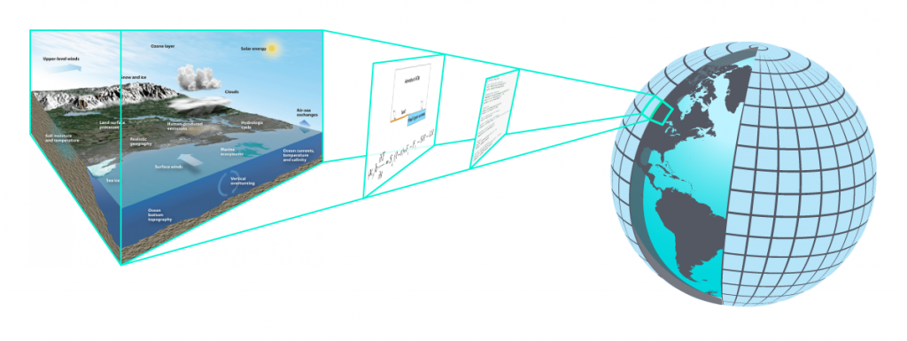
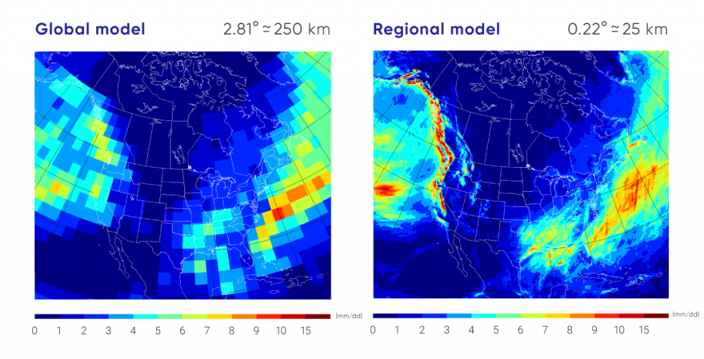
However, for other applications, global climate model projections are not adequate, as they typically have horizontal spatial resolution, or grid spacing, of 100 km or coarser (see Figure 3.2 for explanation of model characteristics) (e.g., Charon, 20143). As an example, when using climate projections to drive a detailed hydrological model at the scale of a drainage basin, one needs values of future climate variables at a scale that respects local topographic, coastal, and other features, and represents high-frequency variability and extremes. Users of climate projections must therefore first evaluate whether they really need high-resolution climate scenarios or whether they could make effective use of lower-resolution climate change scenarios. Higher resolution, in and of itself, does not necessarily indicate higher-quality or more valuable climate information. But, for many applications, higher resolution may be necessary, and can also facilitate better understanding among, and communication to, users. A caution, however, is that internal climate variability is reduced by averaging results over large areas, and so as one goes from global to regional to local scale, internal variability becomes larger, leading to larger uncertainty in projections at the local scale, relative to that at regional or global scale (Hawkins and Sutton, 2009 21).

When climate information at a higher spatial- or temporal-resolution is needed, there are several approaches available to take global climate model projections and “downscale” them to higher resolution for a region of interest (or even a single location). These generally fall into two categories: statistical and dynamical downscaling.

Statistical downscaling is a form of climate model “post-processing” that combines climate model projections with local or regional observations to provide climate information with more spatial detail (Maraun et al., 201033; Hewitson et al., 201422). Statistical post-processing methods typically downscale to higher resolution and correct systematic model biases. A simple example is the so-called “delta method,” in which the change in some climate quantity, obtained from a climate model projection, is added to the observed historical value of that quantity. This allows projected changes from different climate models to be used in a consistent manner, since each model’s climatological bias is eliminated. Bias correction is particularly important when using downscaled climate information to drive impact models that depend on crossing absolute thresholds. For example, snow accumulation is sensitive to whether temperature is above or below freezing.

Simple techniques like the delta method may be suitable for some quantities, such as mean temperature, but not for others, such as daily precipitation, for which biases may be manifested differently, in variability, extremes, or dry/wet spells (Maraun et al., 201033). More complex statistical downscaling approaches are required in such cases, making use of detailed high-resolution observational datasets that reflect local topographic influences. These high-resolution data are used to interpolate low-resolution climate change projections to much higher resolution. In some cases, bias correction and other refinements are applied to correct statistical properties such as variances (Werner and Cannon, 201656). Yet other statistical downscaling methods take advantage of observed relationships between large-scale atmospheric circulation patterns, which are often well simulated by climate models, and local variables. By assuming that these statistical relationships remain fixed under a changing climate, climate model projections of circulation patterns can be used to make projections of future climate at a particular location. The statistical relationships introduce some aspects of local climate that may not be well represented in the driving global model (e.g., local topography and proximity to a lake). Fundamentally, all statistical downscaling methods assume that relationships between a model’s historical simulation and observations do not change over time, and that the information provided by the climate model and historical observations at their respective spatial scales is credible. Thus, the quality of statistical downscaling is directly related to the quality and availability of observational data. Recent critical reviews provide more information on the strengths and weaknesses of statistical downscaling and bias correction methods (Hewitson et al., 201422; Maraun, 201632).

Dynamical downscaling involves the use of a regional climate model, which is a physically based climate model (of the same level of complexity as a global model) that operates at high resolution over a limited area. Regional climate models incorporate much the same physical processes and scientific understanding as global climate models and indeed often share much of the same computer code. The important distinction is that regional climate models are driven at their lateral boundaries by output from a global climate model, as shown in Figure 3.10. The regional model also inherits errors and biases that may be present in the global model whose results are provided at the boundaries. The main advantage of dynamical downscaling is that, due to its limited area, a regional model can simulate climate on a much higher resolution than is possible with a global model, using a similar amount of computing effort. This additional detail is often desirable, particularly where the regional model output is used to drive another model (e.g., a hydrological model in which detailed basin geometry, high-frequency precipitation and extremes, and other small-scale features are essential). However, it remains an ongoing research topic to determine whether, and under what conditions, regional models add value relative to the original global model results that are being downscaled. There are no agreed-upon measures for added value (Di Luca et al., 201510; 20168; Scinocca et al., 201645), although the evidence available at the time of the IPCC Fifth Assessment indicated that there is added value in some locations owing to the better representation of topography, land/water boundaries, and certain physical processes, and that extremes are better simulated in high-resolution regional models (e.g., Flato et al., 201314).

Figure-3.10

Comparative resolution of global and regional climate models

The left panel shows a map of North America covered by coloured squares, illustrating the precipitation simulated by a global model for a particular month — the coarse resolution is clearly evident by the large coloured squares. The right panel shows the same map of North America, but this time with monthly precipitation simulated by a 25 km resolution regional model. The colour scales are the same, but in this case the fine detail provided by a regional model is clearly evident, with intense precipitation over the mountain areas of British Columbia, for example.
Figure-3.10

Monthly precipitation simulated by the global model (left) and regional model (right) based on simulations described by Scinocca et al. (2016). The global model results are provided to the regional model along its boundaries, and the regional model recomputes climate in the interior of that limited area domain. The higher-resolution regional model provides more detail, as seen in the simulated precipitation patterns.

Source

Based on simulations described by Scinocca et al. (2016).

An additional advantage of dynamical over statistical downscaling is that physical relationships between different climate variables (such as temperature and precipitation) are maintained. For very-high-resolution dynamical downscaling (at model resolution of a few kilometres), physical processes such as convection can be resolved explicitly and can lead to improved simulation of climate variables such as precipitation extremes. Several recent studies indicate added value, including a dynamical downscaling system that includes a detailed representation of the Great Lakes (Gula and Peltier, 201220), the potential for added value near well-resolved coastlines (Di Luca et al., 20139), and evidence for improved simulation of temperature and precipitation extremes (Curry et al., 2016a6,b7; Erler and Peltier, 201611).

3.5.2

Downscaling results for North America and Canada

Both statistical and dynamical downscaling approaches have been applied and evaluated in many areas of the world. For North America, coordinated dynamical downscaling comparisons have been undertaken as part of the North American Regional Climate Change Assessment Program (NARCCAP: http://www.narccap.ucar.edu/) and the Coordinated Regional Downscaling Experiment (CORDEX: https://na-cordex.org/). For CORDEX, simulations were run at resolutions of approximately 25 km and 50 km. In both NARCCAP and CORDEX, Canadian models are represented. Coordinated experiments like these provide results from different regional climate models, driven at their boundaries by output from different global climate models. They also allow scientists to determine whether regional differences in projected climate change are related to the differences in the global driving models or to differences in the regional downscaling models. However, the CORDEX ensemble is considerably smaller than the CMIP global model ensemble, and studies using the CORDEX ensemble tends to focus on sub-regions rather than on Canada as a whole.

For Canada, regional climate models with smaller domains and higher resolution are being used, particularly by the Ouranos consortium and the Centre pour l’étude et la simulation du climat à l’échelle régionale (ESCER) at the Université du Québec à Montréal. Some of these simulations provide results at 15 km resolution (e.g., https://www.ouranos.ca/en/program/climate-simulation-and-analysis/). Statistical downscaling results are also readily available for Canada (https://www.pacificclimate.org/data/statistically-downscaled-climate-scenarios), with daily temperature and precipitation data at approximately 10 km resolution. These state-of-the-art downscaling approaches (Werner and Cannon, 201656) are driven by multiple global climate model projections. In addition to the more detailed spatial structure, sophisticated statistical downscaling approaches can also provide estimates of future changes in climate extremes and other indices (such as frequency of hot days, growing season length, and drought indices) that are particularly important for certain impact studies (see Chapter 4). Downscaled results can also be used as inputs to impacts models — such as hydrological, crop, and ecosystem models — that are sensitive to variability on small spatial scales and to biases in climate models (Wood et al., 200457).


Section summary

In summary, global Earth system models are necessarily limited in the level of fine spatial detail they can resolve. Techniques such as statistical or dynamical downscaling allow transformation of these large-scale projections to a level of detail better suited to the climate information needs of many local and regional impact studies. It must be noted, however, that uncertainty due to internal climate variability is reduced by area averaging (e.g., averaging over Canada or the globe), and so uncertainty in climate projections is larger as one goes from global to regional to local scale.

Footnotes

  1. Radiative forcing is the net change in the energy balance of the earth system due to an external perturbation. A positive radiative forcing, such as that from the increase in atmospheric greenhouse gases, causes climate warming, whereas a negative radiative forcing causes climate cooling.

References

  1. Arctic Council (2011): Arctic Council Task Force on short-lived climate forcers: progress report and recommendations for ministers; 12 p., <https://oaarchive.arctic-council.org/bitstream/handle/11374/79/3-0a_TF_SPM_recommendations_2May11_final%20%281%29.pdf?sequence=1&isAllowed=y> [17 August 2018].
  2. Burkett, V.R., Suarez, A.G., Bindi, M., Conde, C., Mukerji, R., Prather, M.J., St. Clair, A.L. and Yohe, G.W. (2014): Point of departure; in Climate Change 2014: Impacts, Adaptation, and Vulnerability; Part A: Global and Sectoral Aspects (Contribution of Working Group II to the Fifth Assessment Report of the Intergovernmental Panel on Climate Change), (ed.) C.B. Field, V.R. Barros, D.J. Dokken, K.J. Mach, M.D. Mastrandrea, T.E. Bilir, M. Chatterjee, K.L. Ebi, Y.O. Estrada, R.C. Genova, B. Girma, E.S. Kissel, A.N. Levy, S. MacCracken, P.R. Mastrandrea and L.L. White; Cambridge University Press, Cambridge, United Kingdom and New York, NY, USA, p. 169–194.
  3. Charron, I. (2014): A guidebook on climate scenarios: using climate information to guide adaptation research and decisions; Consortium on regional climatology and adaptation to climate change, Ouranos, Montreal, QC, Canada, 86 p.
  4. Ciais, P., Sabine, C., Bala, G., Bopp, L., Brovkin, V., Canadell, J., Chhabra, A., DeFries, R., Galloway, J., Heimann, M., Jones, C., Le Quéré, C., Myneni, R.B., Piao S., and Thornton, P. (2013): Carbon and other biogeochemical cycles; in Climate Change 2013: The Physical Science Basis (Contribution of Working Group I to the Fifth Assessment Report of the Intergovernmental Panel on Climate Change), (ed.) T.F. Stocker, D. Qin, G.-K. Plattner, M. Tignor, S.K. Allen, J. Boschung, A. Nauels, Y. Xia, V. Bex and P.M. Midgley; Cambridge University Press, Cambridge, United Kingdom and New York, NY, USA, p. 465–570.
  5. Collins, M., Knutti, R., Arblaster, J., Dufresne, J.-L., Fichefet, T., Friedlingstein, P., Gao, X., Gutowski, W.J., Johns, T., Krinner, G., Shongwe, M., Tebaldi, C., Weaver, A.J. and Wehner, M. (2013): Long-term climate change: projections, commitments and irreversibility; in Climate Change 2013: The Physical Science Basis (Contribution of Working Group I to the Fifth Assessment Report of the Intergovernmental Panel on Climate Change), (ed.) T.F. Stocker, D. Qin, G.-K. Plattner, M. Tignor, S.K. Allen, J. Boschung, A. Nauels, Y. Xia, V. Bex and P.M. Midgley; Cambridge University Press, Cambridge, United Kingdom and New York, NY, USA, p. 1029–1136.
  6. Curry, C.L., Tencer, B., Whan, K., Weaver, A.J. and Giguère, M. (2016a): Searching for added value in simulating climate extremes with a high-resolution regional climate model over western Canada; Atmosphere-Ocean, v. 54., p. 364–384. doi:10.1080/07055900.2016.1158146
  7. Curry, C.L., Tencer, B., Whan, K., Weaver, A.J., Giguère, M. and Wiebe, E. (2016b): Searching for added value in simulating climate extremes with a high-resolution regional climate model over western Canada. II: Basin-Scale Results; Atmosphere-Ocean, v. 54, p. 385–402.
  8. Di Luca, A., Argüeso, D., Evans, J.P., de Elía, R. and Laprise, R. (2016): Quantifying the overall added value of dynamical downscaling and the contribution from different spatial scales; Journal of Geophysical Research Atmospheres, v. 121, p. 1575–1590. doi:10.1002/2015JD024009.
  9. Di Luca, A., de Elía, R. and Laprise, R. (2013): Potential added value of RCM’s downscaled climate change signal; Climate Dynamics, v. 40, p. 601–618. doi:10.1007/s00382-012-1415-z
  10. Di Luca, A., de Elía, R. and Laprise, R. (2015): Challenges in the quest for added value of regional climate dynamical down-scaling; Current Climate Change Report, v. 1, p. 10–21. doi:10.1007/s40641-015-0003-9
  11. Erler, A.R. and Peltier, W.R. (2016): Projected changes in precipitation extremes for western Canada based on high-resolution regional climate simulations; Journal of Climate, v. 29, p. 8841–8863. doi:10.1175/JCLI-D-15-0530.1
  12. Euskirchen, E.S., Bennett, A.P., Breen, A.L., Genet, H., Lindgren, M.A., Kurkowski, T.A., McGuire, A.D. and Rupp, T.S. (2016): Consequences of changes in vegetation and snow cover for climate feedbacks in Alaska and northwest Canada; Environmental Research Letters, v. 11, 19 p. doi:10.1088/1748-9326/11/10/105003
  13. Flato, G.M. (2011): Earth system models: An overview. WIREs Climate Change, v. 2, p. 783–800. doi:10.1002/wcc.148
  14. Flato, G., Marotzke, J., Abiodun, B., Braconnot, P., Chou, S.C., Collins, W., Cox, P., Driouech, F., Emori, S., Eyring, V., Forest, C., Gleckler, P., Guilyardi, E., Jakob, C., Kattsov, V., Reason C. and Rummukainen M. (2013): Evaluation of climate models; in Climate Change 2013: The Physical Science Basis (Contribution of Working Group I to the Fifth Assessment Report of the Intergovernmental Panel on Climate Change), (ed.) T.F. Stocker, D. Qin, G.-K. Plattner, M. Tignor, S.K. Allen, J. Boschung, A. Nauels, Y. Xia, V. Bex and P.M. Midgley; Cambridge University Press, Cambridge, United Kingdom and New York, NY, USA, p. 741–866.
  15. Forkel, M., Carvalhais, N., Rödenbeck, C., Keeling, R., Heimann, M., Thonicke, K., Zaehle, S. and Reichstein, M. (2016): Enhanced seasonal CO2 exchange caused by amplified plant productivity in northern ecosystems; Science, v. 351, p. 696–699.
  16. Frölicher, T.L. and Joos, F. (2010): Reversible and irreversible impacts of greenhouse gas emissions in multi-century projections with the NCAR global coupled carbon cycle-climate model; Climate Dynamics, v. 35, p. 1439–1459.
  17. Fyfe, J.C., Meehl, G.A., England, M.H., Mann, M.E., Santer, B.D., Flato, G.M., Hawkins, E., Gillett, N.P., Xie, S.-P., Kosaka, Y. and Swart, N.C. (2016): Making sense of the early-2000s global warming slowdown; Nature Climate Change, v. 6, p. 224–228.
  18. Gillett, N.P., Arora V.K., Zickfeld K., Marshall S.J., Merryfield W.J. (2011): Ongoing climate change following a complete cessation of carbon dioxide emissions; Nature Geoscience, v. 4, p. 83–87.
  19. Goodwin, P., Katavouta, A., Roussenov, V.M., Foster, G.L., Rohling, E.J. and Williams, G. (2018): Pathways to 1.5 °C and 2 °C warming based on observational and geological constraints; Nature Geoscience, v. 11, p. 102–107. doi:10.1038/s41561-017-0054-8
  20. Gula, J. and Peltier, W.R. (2012): Dynamical downscaling over the Great Lakes Basin of North America using the WRF regional climate model: The impact of the Great Lakes System on regional greenhouse warming; Journal of Climate, v. 25, p. 7723–7742. doi.org/10.1175/JCLI-D-11-00388.1
  21. Hawkins, E. and Sutton, R. (2009): The potential to narrow uncertainty in regional climate predictions; Bulletin of the American Meteorological Society, v. 90, p. 1095–1107. doi:10.1175/2009BAMS2607.1
  22. Hewitson, B.C., Daron, J., Crane, R.G., Zermoglio, M.F. and Jack, C. (2014): Interrogating empirical-statistical downscaling; Climatic Change, v. 122, p. 539–554.
  23. IPCC [Intergovernmental Panel on Climate Change] (2013): Summary for Policymakers; in Climate Change 2013: The Physical Science Basis (Contribution of Working Group I to the Fifth Assessment Report of the Intergovernmental Panel on Climate Change), (ed.) T.F. Stocker, D. Qin, G.-K. Plattner, M. Tignor, S.K. Allen, J. Boschung, A. Nauels, Y. Xia, V. Bex and P.M. Midgley; Cambridge University Press, Cambridge, United Kingdom and New York, NY, USA, p. 3–29.
  24. IPCC [Intergovernmental Panel on Climate Change] (2014): Climate Change 2014: Synthesis Report (Contribution of Working Groups I, II and III to the Fifth Assessment Report of the Intergovernmental Panel on Climate Change), (ed.) Core Writing Team, R.K. Pachauri and L.A. Meyer; IPCC, Geneva, Switzerland, 151 p.
  25. Jones, C., Robertson, E., Arora, V., Friedlingstein, P., Shevliakova, E., Bopp, L., Brovkin, V., Hajima, T., Kato, E., Kawamiya, M., Liddicoat, S., Lindsay, K., Reick, C.H., Roelandt, C., Segschneider, J. and Tjiputra, J. (2013): Twenty-first-century compatible CO2 emissions and airborne fraction simulated by CMIP5 earth system models under four Representative Concentration Pathways; Journal of Climate, v. 26, p. 4398–4413.
  26. Kashiwase, H., Ohshima, K.I., Nihashi, S. and Eicken, H. (2017): Evidence for ice-ocean albedo feedback in the Arctic Ocean shifting to a seasonal ice zone; Scientific Reports, v. 7, 10 p. doi:10.1038/s41598-017-08467-z
  27. Kharin, V.V., Merryfield, W.J., Boer, G.J. and Lee, W.-S. (2017): A postprocessing method for seasonal forecasts using temporally and spatially smoothed statistics; Monthly Weather Review, v. 145, p. 3545–3561. doi.org/10.1175/MWR-D-16-0337.1
  28. Kirtman, B., Power, S.B., Adedoyin, J.A., Boer, G.J., Bojariu, R., Camilloni, I., Doblas-Reyes, F.J., Fiore, A.M., Kimoto, M., Meehl, G.A., Prather, M., Sarr, A., Schär, C., Sutton, R., van Oldenborgh, G.J., Vecchi G. and Wang, H.J. (2013): Near-term climate change: projections and predictability; in Climate Change 2013: The Physical Science Basis (Contribution of Working Group I to the Fifth Assessment Report of the Intergovernmental Panel on Climate Change), (ed.) T.F. Stocker, D. Qin, G.-K. Plattner, M. Tignor, S.K. Allen, J. Boschung, A. Nauels, Y. Xia, V. Bex and P.M. Midgley; Cambridge University Press, Cambridge, United Kingdom and New York, NY, USA, p. 953–1028. doi:10.1017/CBO9781107415324.023
  29. Knutti, R., Sedláček, J., Sanderson, B.M., Lorenz, R., Fischer, E.M. and Eyring, V. (2017): A climate model projection weighting scheme accounting for performance and interdependence; Geophysical Research Letters, v. 44, p. 1909–1918. doi:10.1002/2016GL072012
  30. Le Quéré, C., Andrew, R.M., Friedlingstein, P., Sitch, S., Pongratz, J., Manning, A.C., Korsbakken, J.I., Peters, G.P., Canadell, J.G., Jackson, R.B., Boden, T.A., Tans, P.P., Andrews, O.D., Arora, V.K., Bakker, D.C.E., Barbero, L., Becker, M., Betts, R.A., Bopp, L., Chevallier, F., Chini, L.P., Ciais, P., Cosca, C.E., Cross, J., Currie, K., Gasser, T., Harris, I., Hauck, J., Haverd, V., Houghton, R.A., Hunt, C.W., Hurtt, G., Ilyina, T., Jain, A.K., Kato, E., Kautz, M., Keeling, R.F., Goldewijk, K.K., Körtzinger, A., Landschützer, P., Lefèvre, N., Lenton, A., Lienert, S., Lima, I., Lombardozzi, D., Metzl, N., Millero, F., Monteiro, P.M.S., Munro, D.R., Nabel, J.E.M.S., Nakaoka, S.-I., Nojiri, Y., Padín, A.X., Peregon, A., Pfeil, B., Pierrot, D., Poulter, B., Rehder, G., Reimer, J., Rödenbeck, C., Schwinger, J., Séférian, R., Skjelvan, I., Stocker, B.D., Tian, H., Tilbrook, B., van der Laan-Luijkx, I.T., van der Werf, G.R., van Heuven, S., Viovy, N., Vuichard, N., Walker, A.P., Watson, A.J., Wiltshire, A.J., Zaehle, S. and Zhu, D. (2017): Global carbon budget 2017; Earth System Science Data Discussions, v. 10, p. 405–448. doi:10.5194/essdd-2017-123
  31. MacDougall, A.H., Zickfeld, K., Knutti, R. and Matthews, D. (2015): Sensitivity of carbon budgets to permafrost carbon feedbacks and non-CO2 forcings; Environmental Research Letters, v. 10, 10 p. doi:10.1088/1748-9326/10/12/125003
  32. Maraun, D. (2016): Bias correcting climate change simulations — a critical review; Current Climate Change Reports, v. 2, p. 211–220.
  33. Maraun, D., Wetterhall, F., Ireson, A.M., Chandler, R. E., Kendon, E.J., Widmann, M., Brienen, S., Rust, H. W., Sauter, T., Themeßl, M., Venema, V.K.C., Chun, K.P., Goodess, C.M., Jones, R.G., Onof, C., Vrac, M. and Thiele-Eich, I. (2010): Precipitation downscaling under climate change: Recent developments to bridge the gap between dynamical models and the end user; Reviews of Geophysics, v. 48, 34 p. doi:10.1029/2009RG000314
  34. Matsuno, T., Maruyama, K. and Tsutsui, J. (2012): Stabilization of atmospheric carbon dioxide via zero emissions — an alternative way to a stable global environment. Part 1: examination of the traditional stabilization concept; Proceedings Japan Academic Series B Physical Biological Science, v. 88, p. 368–384.
  35. Matthews, H.D. and Caldeira, K. (2008): Stabilizing climate requires near-zero emissions; Geophysical Research Letters, v. 35, 5 p. doi:10.1029/2007GL032388
  36. Merryfield, W.J., Lee, W.-S., Wang, W., Chen, M. and Kumar, A. (2013): Multi-system seasonal predictions of Arctic sea ice, Geophysical Research Letters, v. 40, p. 1551–1556. doi:10.1002/grl.50317
  37. Millar, R., Fuglestvedt, J., Friedlingstein, P., Rogelj, J., Grubb, M., Matthews, H.D., Skeie, R.B., Forster, P.M., Frame, D.J. and Allen, M.R. (2017): Emission budgets and pathways consistent with limiting warming to 1.5° C; Nature Geoscience, v. 10, p. 741–747.
  38. Morice, C.P., Kennedy, J.J., Rayner, N.A., Jones and Jones, P.D. (2012): Quantifying uncertainties in global and regional temperature change using an ensemble of observational estimates: The HadCRUT4 data set; Journal of Geophysical Research, v. 117. doi:10.1029/2011JD017187
  39. Myhre, G., Shindell, D., Bréon, F.-M., Collins, W., Fuglestvedt, J., Huang, J., Koch, D., Lamarque, J.-F., Lee, D., Mendoza, B., Nakajima, T., Robock, A., Stephens, G., Takemura, T. and Zhang, H. (2013): Anthropogenic and natural radiative forcing; in Climate Change 2013: The Physical Science Basis (Contribution of Working Group I to the Fifth Assessment Report of the Intergovernmental Panel on Climate Change), (ed.) T.F. Stocker, D. Qin, G.-K. Plattner, M. Tignor, S.K. Allen, J. Boschung, A. Nauels, Y. Xia, V. Bex and P.M. Midgley; Cambridge University Press, Cambridge, United Kingdom and New York, NY, USA, p. 659–740. doi:10.1017/ CBO9781107415324.018
  40. Nakicenovic, N., Alcamo, J., Davis, G., de Vries, B., Fenhann, J., Gaffin, S., Gregory, K., Grübler, A., Jung, T.Y., Kram, T., La Rovere, E.L., Michaelis, L., Mori, S., Morita, T., Pepper, W., Pitcher, H., Price, L., Riahi, K., Roehrl, A., Rogner, H.-H., Sankovski, A., Schlesinger, M., Shukla, P., Smith, S., Swart, R., van Rooijen, S., Victor, N. and Dadi, Z. (2000): Special report on emissions scenarios (Contribution of Working Group III to the Fifth Assessment Report of the Intergovernmental Panel on Climate Change); Cambridge University Press, Cambridge, United Kingdom and New York, NY, USA, 599 p.
  41. Riahi, K., van Vuuren, D.P., Kriegler, E., Edmonds, J., O’Neil, B.C., Fujimori, S., Bauer, N., Calvin, K., Dellink, R., Fricko, O., Lutz, W., Popp, A., Cuaresma, J.C., KC, S., Leimbach, M., Jiang, L., Kram, T., Rao, S., Emmerling, J., Ebi, K., Hasegawa, T., Havlik, P., Humpenöder, F., Da Silva, L.A., Smith, S., Stehfest, E., Bosetti, V., Eom, J., Gernaat, D., Masui, T., Rogelj, J., Strefler, J., Drouet, L., Krey, V., Luderer, G., Harmsen, M., Takahashi, K., Baumsark, L., Doelman, J.C., Kainuma, M., Klimont, Z., Marangoni, G., Lotze-Campen, H., Obersteiner, M., Tabeau, A. and Tavoni, M. (2017): The shared socioeconomic pathways and their energy, land use, and greenhouse gas emissions implications: An overview; Global Environmental Change, v. 42, p. 153–168. doi.org/10.1016/j.gloenvcha.2016.05.009
  42. Rogelj, J., Schaeffer, M., Friedlingstein, P., Gillett, N.P., Van Vuuren, D.P., Riahi, K., Allen, M. and Knutti, R. (2016): Differences between carbon budget estimates unravelled; Nature Climate Change, v. 6, p. 245–252.
  43. Sanderson, B.M., Wehner, M. and Knutti, R. (2017): Skill and independence weighting for multi-model assessments; Geoscientific Model Development, v. 10, p. 2379–2395. doi:10.5194/gmd-10-2379-2017
  44. Schuur, E.A.G., Bockheim, J., Canadell, J.G., Euskirchen, E., Field, C.B., Goryachkin, S.V., Hagemann, S., Kuhry, P., Lafleur, P.M., Mazhitova, H.L.G., Nelson, F.E., Rinke, A., Romanovsky, V.E., Shiklomanov, N., Tarnocai, C., Venevsky, S., Vogel, J.G. and Zimov, S.A. (2008): Vulnerability of permafrost carbon to climate change: implications for the global carbon cycle; BioScience, v. 58, p. 701–714. doi:10.1641/B580807
  45. Scinocca, J.F., Kharin, V.V., Jian, Y., Qian, M.W., Lazare, M., Solheim, L. and Flato, G.M. (2016): Coordinated global and regional climate modelling; Journal of Climate, v. 29, p. 17–35. doi:10.1175/JCLI-D-15-0161.1
  46. Shepherd, T.G. (2014): Atmospheric circulation as a source of uncertainty in climate change projections; Nature Geoscience, v. 7, p. 703–708. doi:10.1038/ngeo2253
  47. Sigmond, M., Fyfe, J.C., Flato, G.M., Kharin, V.V. and Merryfield, W.J. (2013): Seasonal forecast skill of Arctic sea ice area in a dynamical forecast system; Geophysical Research Letters, v. 40, p. 529–534. doi:10.1002/grl.50129
  48. Smith, S.M., Lowe, J.A., Bowerman, N.H., Gohar, L.K., Huntingford, C. and Allen, M.R. (2012): Equivalence of greenhouse-gas emissions for peak temperature limits; Nature Climate Change., v. 2, p. 535–538.
  49. Stuecker,M.F., Bitz, C.M., Armour, K.C., Proistosescu, C., Kang, S.M., Xie, S-P., Kim, D., McGregor, S., Zhang, W., Zhao, S., Cai, W., Dong, Y., Jin, F-F. (2018): Polar amplification dominated by local forcing and feedbacks. Nature Climate Change, v. 8, p. 1076-1081.
  50. Taylor, K.E., Stouffer, R.J. and Meehl, G.A. (2012): An overview of CMIP5 and the experimental design; Bulletin American Meteorological Society, v. 93, p. 485–498. doi:10.1175/BAMS-D-11-00094.1
  51. Tokarska K.B. and Gillett, N.P. (2018): Cumulative carbon emissions budgets consistent with 1.5 °C global warming; Nature Climate Change, v. 8, p. 269–299.
  52. Tokarska, K.B., Gillett, N.P., Weaver, A.J., Arora, V.K. and Eby, M. (2016): The climate response to five trillion tonnes of carbon; Nature Climate Change, v. 6, p. 851–855.
  53. UNFCCC [United Nations Framework Convention on Climate Change] (2015): The Paris Agreement; United Nations Framework Convention on Climate Change https://unfccc.int/sites/default/files/english_paris_agreement.pdf [17 August 2018].
  54. van Vuuren, D.P., Edmonds, J., Kainuma, M., Riahi, K., Thomson, A., Hibbard, K., Hurtt, G.C., Kram, T., Krey, V., Lamarque, J.-F., Masui, T., Meinshausen, M., Nakicenovic, N., Smith, S.J. and Rose, S.K. (2011): The representative concentration pathways: An overview; Climatic Change, v. 109, p. 5–31.
  55. Weigel, A.P., Knutti, R., Liniger, M.A. and Appenzeller, C. (2010): Risks of model weighting in multimodel climate projections; Journal of Climate, v. 23, p. 4175–4191. doi: 10.1175/2010JCLI3594.1
  56. Werner, A.T. and Cannon, A.J. (2016): Hydrologic extremes: An intercomparison of multiple gridded statistical downscaling methods; Hydrology and Earth System Sciences, v. 20, p. 1483–1508. doi:10.5194/hess-20-1483-2016
  57. Wood, A.W., Leung, L.R., Sridhar, V. and Lettenmaier, D.P. (2004): Hydrologic implications of dynamical and statistical approaches to downscaling climate model outputs; Climatic Change, v. 62, p. 189–216.
Next

Changes in Temperature and Precipitation Across Canada